True Stress - True Strain Curve: Part Four
Abstract
This article examines the mathematical relationships and material constants used in analyzing stress-strain behavior during work hardening. It focuses on the strain-hardening exponent (n) and strength coefficient (K), explaining their roles in various equations, particularly the Ludwig equation. The discussion includes detailed analysis of power curve relations, material-specific variations, and practical applications in metal deformation calculations, providing essential insights for materials engineering and metal forming processes.
Introduction to Flow Curves and Material Constants
The flow curve of metals in the uniform plastic deformation region can be expressed through a simple power curve relation:
 ...(10)
where n represents the strain-hardening exponent and K is the strength coefficient. When plotted on a log-log scale, true stress and true strain up to maximum load will yield a straight line if the data satisfies Equation (10).
Figure 2. Log/log plot of true stress-strain curve
Understanding Strain-Hardening Parameters
The linear slope of this logarithmic plot equals n, while K represents the true stress at ε = 1.0 (corresponding to θ = 0.63). The strain-hardening exponent ranges from n = 0 (indicating a perfectly plastic solid) to n = 1 (representing an elastic solid). Most metals exhibit n values between 0.10 and 0.50, see Table 1.
Figure 3. Various forms of power curve s=K* e n
Table 1. Values for n and K for metals at room temperature
| Metal | Condition | n | K, psi |
| 0,05% C steel | Annealed | 0,26 | 77000 |
| SAE 4340 steel | Annealed | 0,15 | 93000 |
| 0,60% C steel | Quenched and tempered 1000oF | 0,10 | 228000 |
| 0,60% C steel | Quenched and tempered 1300oF | 0,19 | 178000 |
| Copper | Annealed | 0,54 | 46400 |
| 70/30 brass | Annealed | 0,49 | 130000 |
Material-Specific Applications and Variations
The strain-hardening rate (dσ/dε) differs from the strain-hardening exponent. This relationship can be expressed as:
or
 ...(11)
Advanced Equations and Deviations
Equation (10), while useful, is not universally applicable. Significant deviations frequently occur, particularly at low strains (10⁻³) or high strains (ε»1.0). These deviations manifest in several important ways:
Common Deviations in Log-Log Plots
When plotting Equation (10) on a log-log scale, one frequent deviation results in two distinct straight lines with different slopes. In cases where data doesn't conform to Equation (10), it may instead follow the relationship:
 ...(12)
Here, Datsko's research demonstrates that ε₀ represents the material's strain hardening accumulated before the tension test.
The Ludwig Equation
A significant modification to the basic relationship is the Ludwig equation:
 ...(13)
In this equation, σ₀ represents the yield stress, while K and n maintain their original definitions from Equation (10). The Ludwig equation offers a more accurate representation since it accounts for non-zero stress at zero strain, addressing a key limitation of Equation (10).
Special Cases and Material-Specific Variations
Morrison's work provides a method for determining σ₀ through the intersection of the strain-hardening point and the elastic modulus line. For specific materials like austenitic stainless steel, which show marked deviations at low strains, the relationship can be expressed as:

where:
- eK approximates the proportional limit
- n1 represents the slope of stress deviation from Equation (10) plotted against ε
Plastic Strain Considerations
For all equations (10-13), the true strain term should properly represent the plastic strain:
ep= etotal- eE= etotal- s/E
Access Thousands of Stress-Strain Diagrams Now!
Total Materia Horizon includes a unique collection of stress-strain curves of metallic and nonmetallic materials. Both true and engineering stress curves are given, for various strain rates, heat treatments and working temperatures where applicable.
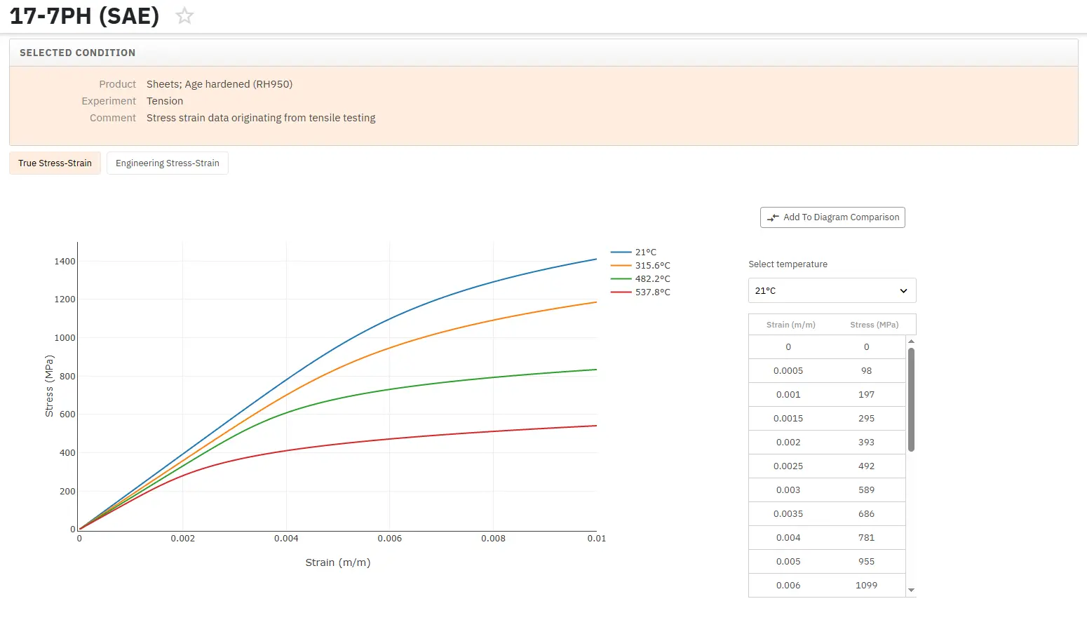
Get a FREE test account at Total Materia Horizon and join a community of over 500,000 users from more than 120 countries.