Control of Sulfur in Melts

Sulfur (S) is a typical metalloid. The radius of sulfur atom is 1.05 Å. It easily acquires two electrons to form an ion S^2-. The coefficient of diffusion of sulfur in liquid iron is 0.74x10^-4, 13x10^-4, 1.9x10_-5 cm/s, according to various experimental data. Sulfur has a strong surface activity both in binary (Fe-S) and ternary (Fe-C-S, Fe-Si-S) alloys. It has been concluded from the results of numerous studies that sulfur can exist in two forms in molten iron: in one case it forms an interstitial solution, and in other partially substitutional solutions. It has been found that the activity of sulfur increase substantially when carbon and silicon are present in the melt. This explains why pig iron can be desulfurized more readily than steel.

A good understanding of the desulphurization of hot metal and liquid steel has been developed in terms of slag-metal reactions, based on a number of studies of the partition of sulfur between liquid slag and liquid iron. These results show that a highly basic slag, high temperature and reducing conditions enhance desulphurization via slag-metal reactions.

 

Sulfur Equilibrium between Liquid Iron and Slag

The desulphurization of liquid iron with slag may be examined on the basis of the following reaction (1), in which the equilibrium constant can be expressed by equation (2).

[S] + (O2-) = (S2-) + [O] .......... (1)

log K₁ = a_s^2-. a_o / a_s. a_o^2- .......... (2)

where,

• a_o, a_s: the activities of oxygen and sulfur in liquid iron, respectively
• a_o^2-, a_s^2-: the activities of oxygen and sulfur ions in slag, respectively.

The sulfur partition ratio between metal and slag is given by equation (3) according to reaction (1).

L_S = (wt%S) / [wt%S] = K₁ • a_o^2- • f_s / a_o • f_s^2- .......... (3)

where,

• f_s, f_s^2- : the activity coefficients of sulfur in liquid iron and slag, respectively.

Since the values of K₁, a_o^2- and f_s^2- cannot be determined experimentally, the sulfide capacity is defined as equation (5) on the basis of reaction (4) and is utilized for the examination of desulphurization in iron and steel making processes.

½ S₂ + (O_2-) = (S^2-) + ½ O₂ .......... (4)

C_S = (wt%S) • (P_O2 / Ps)½ = K₄ a_o2- / f_s^2- .......... (5)

where,

• P_O2 and P_s are the oxygen and sulfur partial pressure in atm;
• K₄ the equilibrium constant of reaction (4).

In order to calculate the value of C_S, the equilibrium constants of reactions (6) and (7) are substituted into equation (5), and equation (8) is obtained.

½ O₂ = [O] .......... (6)

½ S₂ = [S] .......... (7)

log C_s = log (wt % S) a_o / a_s + 936 / T-1.375 .......... (8)

By the use of the interaction coefficients of sulfur and oxygen in liquid iron, the values of C_S can be calculated from equation (8).

As an illustration, the calculation of sulfide capacity (C_S) has been given for CaO-MgO-Al₂O₃-SiO₂ ladle slags.

In order to examine the relationship between C_S and composition of slag, the following relationship is assumed to hold at certain temperatures.

log C_S = α (N_CaO + K_MgO • N_MgO + K_Al2O3• N_Al2O3 + K_SiO2 • N_SiO2)+ β .......... (9)

where:

• α, β: the constants
• Ni, Ki: the mole fraction and the lime equivalent coefficient of i-component in the slag phase, respectively.

At 1600°C, the values of K_MgO, K_Al2O3 and K_SiO2 determined by trial and error are 0.1, -0.8 and -1.0, respectively. As shown in Figure 1, there are linear relations between log C_s and (N_CaO + 0.1 N_MgO – 0.8 N_Al2O3 – N_SiO2) at 1575, 1600 and 1650°C.

 

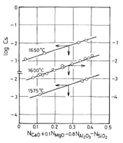
Figure 1: Plot of the log C_s against N_CaO + 0.1N_MgO – 0.8N_Al2O3 – N_SiO2 at 1575, 1600 and 1650°C

The three lines obtained by the method of least squares are shown in the figure. The intercepts of the lines were determined by the use of the slope at 1600°C because the most runs were done at this temperature. The following equation was obtained as a function of temperature.

log C_S = 3.44 (N_CaO +0.1N_MgO – 0.8N_Al2O3 – N_SiO2) - 9894 / T+2.05 .......... (10)

The observed values of log C_S with the correlation coefficient (R) of 0.99 and the standard deviation (σ) of 0.044 can well be expressed by the above equation.

On the other hand, log L_S may be expressed by the following general equation derived from equations. (3), (8) and (10).

log L_S = α ∑ K_i•N_i - log [wt%O] - β .......... (11)

where,

• ∑ K_i•N_i = N_CaO +0.1N_MgO – 0.8N_Al2O3 – N_SiO2.

The experimental data were arranged by the method of least squares according to equation (11) and the following relationship was obtained.

log L_S = 3.44 ∑ K_i•N_i - log [wt% O] - 10 980 / T+3.50 .......... (12)

 

Relationship Between Sulfide Capacity and Theoretical Optical Basicity

Duffy and Ingram defined the theoretical optical basicity (Λ) as follows:

Λ = ∑ (x_i / f_i) .......... (13)

where, x_i, f_i : the equivalent cationic fraction and the basicity moderating parameter for the constituent cation i, respectively.

It was verified by them that f_i can be expressed by the Pauling's electronegativity x_i as follows:

f_i =1.36 (x_i -0.26) .......... (14)

It was also found by Duffy and Ingram that log C_S are linearly correlated to the theoretical optical basicity.

As an illustration of the above mentioned the experimental results performed on ladle CaO-MgO-Al₂O₃-SiO₂ slags has been given. The values of log C_S are plotted against the optical basicities at 1575, 1600 and 1650°C, as shown in Figure 2.

 

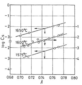
Figure 2: Plot of log CS against theoretical optical basicity Λ

The slopes and intercepts of the lines were determined by the method of least squares, and the following linear relationship was obtained as a function of temperature.

log C_S = 14.20Λ - 9 894 / T -7.55 .......... (15)

As described above, it can be seen that both the sum of lime equivalent and the optical basicity are able to be used as parameters for the representation of sulfide capacity. From the relationship between these two parameters, the linear equation (16) from regression was obtained.

Λ = 0.24(N_CaO + 0.1N_MgO – 0.8N_Al2O3 – N_SiO2) + 0.67 .......... (16)

The correlation coefficient (R) is larger than 0.99, and the standard deviation (σ) is smaller than 0.01. This shows that the two parameters have almost the same character for the representation of sulfide capacity of slag.

 

Equilibrium of Oxygen Partition between Metal and Slag

It is well known that the oxygen potential exerts a large influence on the sulfur partition between metal and slag. The equilibrium of reaction (17) was determined by the use of the value of the equilibrium constant (18) reported in literature.

(FeO) = [Fe] + [O] .......... (17)

log K₁₇ = log a_o / a_FeO = -6 150 / T + 2.604 .......... (18)

Equation (18) may be modified to the following equation.

log [wt%O] = log N_FeO + log γ_FeO - log f_o - 6 150 / T + 2.604 .......... (19)

where γ_FeO is the activity coefficient of FeO on the basis of mole fraction.

Since log γ_FeO is a function of temperature and slag composition, log [wt%O] can be expressed by an equation including the term of log N_FeO, then the following relationship was obtained.

log [wt%O] = 0.905 log N_FeO -0.15 ∑ K_i•N_i - 6 340 / T + 3.115 .......... (20)

where, ∑ K_i•N_i = N_CaO + 0.1N_MgO – 0.8N_Al2O3 – N_SiO2.

As shown in Figure 3, the observed values of log [wt% O] agree well with the values calculated from the equation (20). By substituting equation (20) into equation (12), equation (21) is derived:

log LS = 3.59 ∑ K_i•N_i -0.905 log N_FeO – 4 640 / T + 0.385 .......... (21)

The above equation can conveniently be used for the estimation of the sulfur partition between liquid iron and slag in which the oxygen content in liquid iron is not analyzed. Next, the values of γ_FeO calculated from the equation (19) were arranged by the way similar to that described previously, and the following relationship was obtained.

 

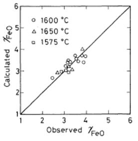
Figure 3: Comparison of the observed log [wt%O] with calculated log [wt%O] from the equation (20)