Creep and Stress Rupture Properties
Abstract
This comprehensive examination explores creep behavior and stress rupture properties in materials, focusing on time-dependent deformation under load at elevated temperatures. The article details testing methodologies, analysis of creep curves, and practical applications in engineering design. Key aspects include the relationship between stress and temperature in creep behavior, mathematical models for predicting material performance, and the significance of various testing parameters in determining material lifetime predictions.
Understanding Creep Fundamentals
Creep is defined as the time-dependent strain that occurs under load at elevated temperature and operates in most applications of heat-resistant high-alloy castings at normal service temperatures. In time, creep may lead to excessive deformation and even fracture at stresses considerably below those determined in room temperature and elevated-temperature short-term tension tests.
Design Considerations and Limiting Factors
When the rate or degree of deformation is the limiting factor, the design stress is based on the minimum creep rate and design life after allowing for initial transient creep. The stress that produces a specified minimum creep rate of an alloy or a specified amount of creep deformation in a given time (for example, 1% of total 100,000 h) is referred to as the limiting creep strength, or limiting stress.
Testing Methodologies
Stress rupture testing complements creep testing and helps determine necessary section sizes to prevent component creep rupture. Long-term creep and stress-rupture values (e.g., 100,000 h) are often extrapolated from short-term tests. Both extrapolated and directly determined property values typically provide accurate information about high-temperature parts' operating life.
Material Behavior Prediction Challenges
The actual material behavior often proves difficult to predict accurately due to:
- Complexity of service stresses
- Variations in application versus idealized conditions
- Uni-axial loading conditions in standard tests
- Attenuating factors including cyclic loading, temperature fluctuations, and corrosion-related metal loss
Creep Testing Procedures
During creep testing, tensile specimens undergo either constant load or stress at constant temperature. Constant load tests primarily provide information for specific engineering applications, while constant stress tests aid in understanding creep mechanisms.
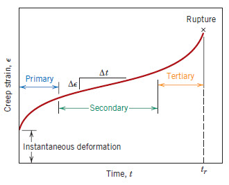
Figure 1: A typical creep curve
Stages of the Creep Curve
The typical creep curve exhibits three distinct stages:
- Primary creep: Increasing creep resistance with strain, leading to decreasing creep strain rate
- Secondary (Steady State) creep: Balance between work hardening and recovery processes, resulting in minimum constant creep rate
- Tertiary creep: Accelerating creep rate due to accumulating damage, potentially leading to creep rupture
Engineering Design Standards
Two commonly used standards include:
- Stress producing 0.0001% creep rate per hour (1% in 10,000 hours)
- Stress producing 0.00001% creep rate per hour (1% in 100,000 hours)
Mathematical Analysis
The minimum secondary creep rate follows the Arrhenius equation: ε= dε/dt = Kσn exp(- Q/RT); for T=const, dε/dt = Kσn
Where: T - temperature [K] tr - time to rupture [h] K - creep constant n - creep exponent (varying from 3-8, typically 5) σ - applied stress/nominal stress Q - activation energy for creep R - gas constant (8,314 J/mol K)
Critical Temperature Considerations
The critical temperature for creep is 40% of the melting temperature in Kelvin: If T>0.40Tm then creep is likely.
Testing Applications and Parameters
Most metallic materials undergo uni-axial tensile mode testing, while brittle materials may require uni-axial compression tests. The minimum creep rate serves as a crucial design parameter for long-life applications, while rupture lifetime becomes paramount for short-life components.
Rupture Life Predictions
The Larson-Miller Time-temperature parameter, derived from stress and temperature dependence of creep rate or rupture time, is expressed as: PLM= T [21.577+ log (tr)]
Access Creep Properties of Thousands of Materials Now!
Total Materia Horizon includes the largest database of creep data such as yield stress and creep rupture strength at different temperatures, for thousands of metallic alloys and polymers.
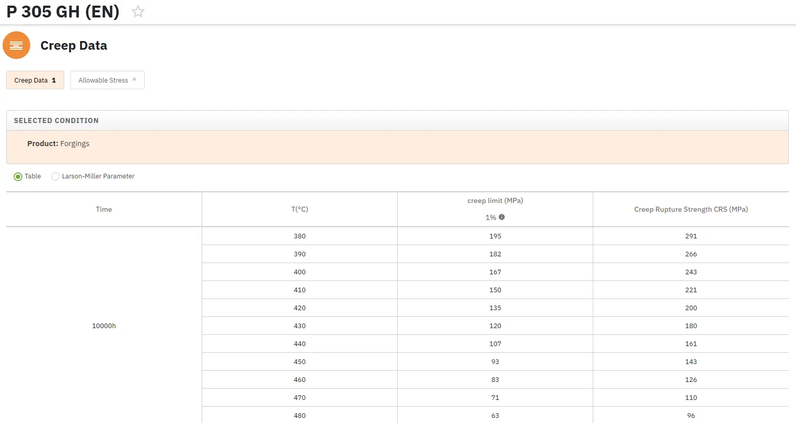
Get a FREE test account at Total Materia Horizon and join a community of over 500,000 users from more than 120 countries.